How residual connections enable surprise in language models

⚠️ Work in Progress: This post is a draft and subject to change.

Language models (LM) rely on momentum, where the present tokens set the linguistic and semantic direction of the next token to be generated. An intelligent model should be able to pivot freely. Yet today’s best models can get caught flat-footed. We’ll define a juke point, where the interpretation of a sentence changes abruptly and potentially derails the LLM.

Consider this funny sentence:

The old man the boats.

Can you spot the subject and verb? Here, “old” is the subject and “man” is the verb, or with part of speech tags: “The old^NOUN man^VERB the boats.”

This oddity is a garden path sentence—a grammatical sentence that initially leads the reader toward an incorrect interpretation.

We’ll focus on this sentence for now, but because it is a well known garden path sentence, LLMs have been trained to parse it correctly.

The conditional probability \(P(\text{man} \mid \text{The old})\) is high because “The old man” is a likely beginning, e.g., “The old man is snoring.”

But what trips up the model is that \(P(\text{the} \mid \text{The old man})\) is quite low, making “the” unlikely to be generated next. In short, there are at least $k$ more likely next tokens and “the” is not likely considered as a possible candidate. We can write this as $P(\text{the} \mid \text{The old man}) < \delta_{\text{top-}k}$, where $\delta_{\text{top-}k}$ is a threshold cutoff for the $k$ most likely tokens.

This allows us to formally define a “juke point” $i = i_{\text{juke}}$ in a sentence, where the continuation probability spikes downward. Specifically, let’s denote the sentence string as $x$, $x[i]$ to indicate the $i\text{th}$ token starting from 0, and $x[:i]$ to indicate the tokens preceding $x[i]$. For example, with $x = “\text{The old man the boats.}”$, we have $x[:3] = “\text{The old man }”$ and $x[3] = “\text{the}”$. We’re interested in sentences $x$ such that for some $i$ we encounter a steep drop \(P(x[i] \mid x[:i]) < \delta_{\text{top-}k}\) yet the full sentence is still grammatically and semantically valid.

The surprise stems from a phase transition. The part of speech (POS) tags shift from “The old^ADJ man^NOUN” to “The old^NOUN man^VERB” and the parsing must jump from noun phrase to clause.

"The young kid gravity."
Giacomond by Quint Buchholz
Licensed under CC BY-SA 4.0

To help understand this, we appeal to the phenomenon of bertology, the idea that LLM layers stratify by linguistic abstraction—from token to POS, to phrase, to clause, to meaning. While often discussed in the context of encoders, this abstraction also holds for LLMs.

In order for such phase transitions to occur, token-level information must be preserved. If higher layers discarded token-specific detail, garden path sentences would become impossible to generate. For example, the shift from [ARTICLE] [ADJ] [NOUN] to [ARTICLE] [NOUN] [VERB] is meaningless without specific, direct token context.

This implies that the model’s conditional probability distribution is sensitive to compression. Explicitly, in full generality we may consider

\[P(y | x) = P(y | \phi(x))\]

where $\phi$ is any function that preserves the equation. It can represent data compression, a stream of reasoning tokens, postprocessing, coordinates induced by manifold learning, or re-organization into an appropriate data structure. What we observe is that $\phi$ must be nearly lossless—a semantic description and parse tree cannot suffice. From a Kolmogorov complexity viewpoint, language is already nearly incompressible. In particular, if we consider each word and its various senses (e.g. “old” could be an adjective or noun) we may find ourselves needing to backtrack to an alternative sense, and therefore $\phi$ cannot make a greedy selection without loss.

Thus, the ability to generate garden path sentences requires superposition across linguistic categories—token, POS, parse, and semantics—especially in the final logit layer. That is, the final hidden vector $h_L$ determining the next token distribution $P(y | x) = F(h_L)$ must contain these \(h_L = h_{\text{tokens}} + h_{\text{POS tags}} + h_{\text{parse tree}} + \cdots\)
Since layers are modular by design, this induces superposition at every layer.

As Wittgenstein put it:

“…if a thing can occur in a state of affairs, the possibility of the state of affairs must be written into the thing itself.” (TLP, 2.012)

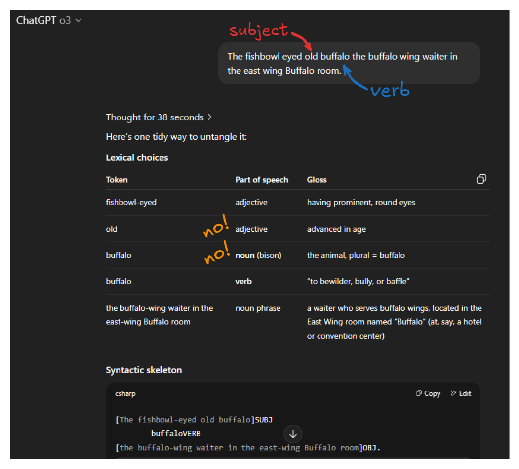
Now, we present some real evidence. We need to make up a garden path sentence unseen in model training and ask an LLM to explain it. This is a fun excerise in its own right. I call this one a Barry Sanders sentence because it uses the model’s own training bias against itself:

As a verb, buffalo means “to bully or overawe”.

The Role of Residual Connections

Enter the residual connection.

The residual connection is not just a training hack for gradient based learning or a scaffold to stabilize corrections. It structurally enables this superposition by ensuring that token-level data remains accessible throughout the network. Without it, the model would play the “telephone game,” eroding token-level distinctions and collapsing under the weight of abstraction.

In lore, the residual connection is often justified as:

1. A mechanism for gradient stability (mitigating vanishing/exploding gradients)
2. A structural way to avoid enforced complexity—an architectural Occam’s Razor

But the garden path sentence gives a semantic justification: the residual connection enables the model to keep a foot in the local while reaching for the global.

A comprehensive LLM walkthrough for the residual connection in context.

Sampling

It’s important to keep in mind that LLMs don’t simply take the highest probability token. Instead, they use a sampler that uses the conditional probability $P(y \mid x)$ as well as strategy to generate tokens. However, most samplers do truncate to a $\text{top-}k$ set of tokens.

We are looking at Zipf’s Law. Ignoring the tail preserves the distribution, so that KL divergence between common crawl and generated text is 0. However, this indicates that equality in probability is easier than passing a Turing test.

Embeddings and Logical Form

This insight also touches on word embeddings (e.g., Word2Vec). It’s often said:

“You shall know a word by the company it keeps.”

Yet this runs aground deep in the Zipfian tail. Wittgenstein again:

“If two objects have the same logical form, the only distinction between them… is that they are different.” (TLP, 2.0233)

In many embedding spaces, “king,” “carpenter,” and “man” blur into one. But the mostly forgotten, fifth sense of a word—one deemed too esoteric for Webster’s dictionary—is not interchangeable with the others. Synonyms often do not share logical form. Our language games are not inefficient; they are precise in edge cases.

Generation vs. Verification

Finally, this analysis touches a deeper tension: generation vs. verification.

Verifying a solution to a Diophantine equation is easy; generating one is hard. Similarly, an encoder can check a sentence’s acceptability (e.g., via a CoLA classifier), but generation must nail the turn at $i_\text{juke}$ without lookahead hints.

Conclusion

The architecture allows for this precision—we therefore rely on the sampler not to fumble it.